Archives February 2024

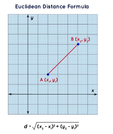
The image illustrates the Euclidean distance formula in a 2D space. It shows two points: (x1,y1) and (x2,y2). The preceding formula calculates the straight-line distance between the two points in a plane.

• Distance metrics – Manhattan (L1): Manhattan distance calculates the sum of absolute differences along each dimension. The higher the metric, the less similar the differences. The following image depicts the Manhattan distance (or L1 distance) between two points in a 2D space, where the distance is measured along the axes at right angles, similar to navigating city blocks in a grid-like street layout:

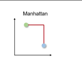
Figure 4.8 – Illustration of Manhattan distance

You might be wondering when to select one metric over another during the development of generative AI applications. The decision on which similarity measure to use hinges on various elements, such as the type of data, the context of the application, and the bespoke demands of the analysis results.

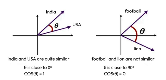
Cosine similarity is preferred over Manhattan and Euclidean distances when the magnitude of the data vectors is less relevant than the direction or orientation of the data. In text analysis, for example, two documents might be represented by highly dimensional vectors of word frequencies. If one document is a longer version of the other, their word frequency vectors will point in the same direction, but the magnitude (length) of one vector will be larger due to the higher word count. Using Euclidean or Manhattan distance would highlight these differences in magnitude, suggesting the documents are different. However, using cosine similarity would capture their similarity in content (the direction of the vectors), de -emphasizing the differences in word count. In this context, cosine similarity is more appropriate, as it focuses on the angle between the vectors, reflecting the content overlap of the documents rather than their length or magnitude.

Euclidean and Manhattan distances are more apt than cosine similarity when the magnitude and absolute differences between data vectors are crucial, such as with consistent scaled numerical data (e.g., age, height, weight, and so on) or in spatial applications such as grid-based pathfinding. While cosine similarity emphasizes the orientation or pattern of data vectors, which is especially useful in highly dimensional, sparse datasets, Euclidean and Manhattan distances capture the actual differences between data points, making them preferable in scenarios where absolute value deviations are significant such as when comparing the medical test results of patients or finding the distance between geographical co-ordinates on earth.

The following is a snippet of code that uses Azure OpenAI endpoints to calculate the similarity between two sentences: “What number of countries do you know?” and “How many countries are you familiar with?” by using embedding model text-embedding-ada-002. It gives a score of 0.95:

import os

import openai

openai.api_type = “azure”

openai.api_base = “https://ak-deployment-3.openai.azure.com/”

openai.api_version = “2023-07-01-preview”

##replace “2023-07-01-preview” with latest version openai.api_key = “xxxxxxxxxxxxxxxxxxxxxxx”

def get_embedding(text, model=”text-embedding-ada-002″):

return openai.Embedding.create(engine=model, input=[text], \ model=model)[‘data’][0][’embedding’]

embedding1 = get_embedding(“What number of countries do you know?”, \

model=’text-embedding-ada-002′)

embedding2 = get_embedding(“How many countries are you familiar \

with?”, model=’text-embedding-ada-002′)

embedding1_np = np.array(embedding1)

embedding2_np = np.array(embedding2)

similarity = cosine_similarity([embedding1_np], [embedding2_np])

print(similarity)

# [[0.95523639]]

Now let us walkthrough a scenario where Cosine Similarity will be preferred over Manhattan distance.

When to Use HNSW vs. FAISS

Use HNSW when:

• High precision in similarity search is crucial.

• The dataset size is large but not at the scale where managing it becomes impractical for HNSW.

• Real-time or near-real-time search performance is required.

• The dataset is dynamic, with frequent updates or insertions.

• Apt for use cases involving text like article recommendation systems

Use FAISS when:

• Managing extremely large datasets (e.g., billions of vectors).

• Batch processing and GPU optimization can significantly benefit the application.

• There’s a need for flexible trade-offs between search speed and accuracy.

• The dataset is relatively static, or batch updates are acceptable.

• Apt for use cases like image and video search.

Note

Choosing the right indexing strategy hinges on several critical factors, including the nature and structure of the data, the types of queries (e.g. range queries, nearest neighbors, exact search) to be supported, and the volume and growth of the data. Additionally, the frequency of data updates (e.g., static vs dynamic) the dimensionality of the data, performance requirements (real-time, batch), and resource constraints play significant roles in the decision-making process.

Similarity measures

Similarity measures dictate how the index is organized, and this makes sure that the retrieved data are highly relevant to the query. For instance, in a system designed to retrieve similar images, the index might be built around the feature vectors of images, and the similarity measure would determine which images are “close” or “far” within that indexed space. The importance of these concepts is two-fold: indexing significantly speeds up data retrieval, and similarity measures ensure that the retrieved data is relevant to the query, together enhancing the efficiency and efficacy of data retrieval systems. Selecting an appropriate distance metric greatly enhances the performance of classification and clustering tasks. The optimal similarity measure is chosen based on the nature of the data input.

In other words, similarity measures define how closely two items or data points are related. They can be broadly classified into distance metrics and similarity metrics. Next, we’ll explore the three top similarity metrics for building AI applications: cosine similarity and Euclidean and Manhattan distance.

• Similarity metrics – Cosine similarity: Cosine similarity, a type of similarity metric, calculates the cosine value of the angle between two vectors, and OpenAI suggests using it for its models to measure the distance between two embeddings obtained from text-embedding-ada-002. The higher the metric, the more similar they are:

Figure 4.6 – Illustration of relatedness through cosine similarity between two words

The preceding image shows a situation where the cosine similarity is 1 for India and the USA because they are related, as both are countries. In the other image, the similarity is 0 because football is not similar to a lion.

• Distance metrics – Euclidean (L2): Euclidean distance computes the straight-line distance between two points in Euclidean space. The higher the metric, the less similar the two points are:

Figure 4.7 – Illustration of Euclidean distance